Insertion Loss and Filter Performance

24 Aug 2021

Background

Filters are almost always a part of electronics design. Design engineers design a filter to achieve certain attenuation in specified frequency range. There are many types of filters, such as high pass, low pass or bandwidth. Popular filter configurations include L-C, C-L-C (π) or L-C-L (T). It is safe to say that when it comes to filter design, the discussion of the subject could easily become a very thick book.

In this article, we only want to discuss one fundamental subject, which is the performance of a filter. The performance of a filter is measured in terms of attenuation, or insertion loss, both of which use the units of dB.

Theory

The best place to start this discussion is CISPR 17, which defines the technical terms of a filter. It also presents detailed explanation of how to measure the insertion loss of a filter.

A filter often provides attenuation to noise in both differential mode and common mode. At low frequency range (often between a few kHz and 1 MHz), noise is predominantly differential mode. When the frequency goes up, common mode noise becomes more dominant.

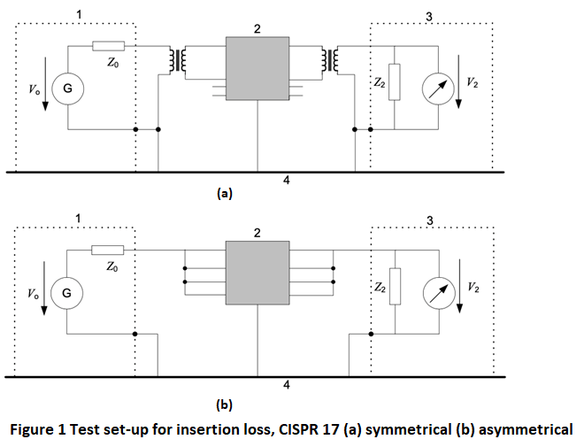
Take a 50Ω/50Ω (source impedance/load impedance) system for instance, CISPR 17 defines two tests to measure the filter performance, which are symmetrical (differential mode) and asymmetrical (common mode). The test set-ups are shown in Figure 1. The signal generator (G) performs a signal sweep between defined frequency range and the voltage over the load (Z2) is measured.

Note that in both cases Z0 and Z2 are 50 Ω. In [1], the author(s) question the 50Ω/50Ω test set-up, arguing that worst-case test set-ups, such as 0.1Ω/100Ω and 100Ω/0.1Ω give better filter performance analysis. It is a valid point, since in reality, a 50Ω/50Ω system barely exists.

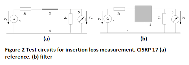
Regardless of the test set-up, the insertion loss is defined as

            Insertion loss = 20log(V20/V2),

Where V20 is the voltage over Z2 before the filter is inserted, V2 is the voltage measurement after the filter is inserted. Test set-ups are shown in Figure 2.

Practical

While the theory sounds easy and straight forward. In order to get a feel of what insertion loss of a filter is all about, here we present a practical example to demonstrate.

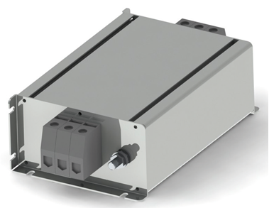
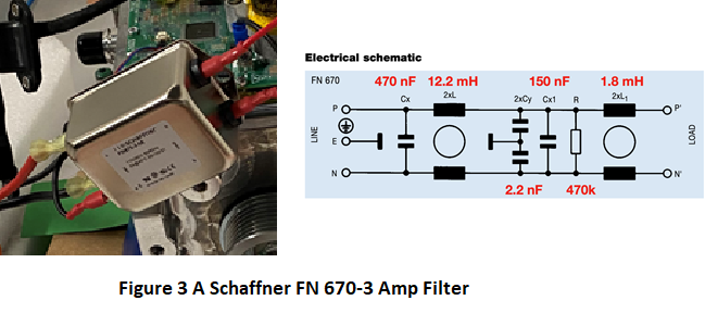
The filter we demonstrate is an off-the-shelf Schaffner part FN 670-3Amp. The filter and its electric schematics are shown in Figure 3.

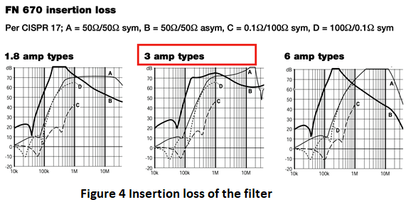
According to the supplier datasheet, the filter performance is shown in Figure 4. As it can be seen, four test set-up results are presented to give the best filter analysis. It should be noted that for set-up C and D, the insertion loss is only performed between 10kHz and 1 MHz. As we mentioned earlier, this is because when frequency goes beyond 1 MHz, common mode noise starts dominating, therefore the measurement results for the symmetrical mode beyond 1 MHz can over predict the filter performance.

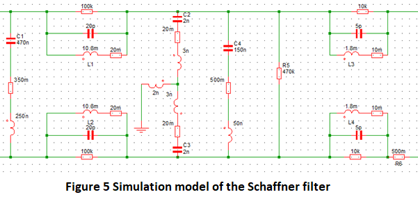
A SPICE based simulation model is then modelled to demonstrate the insertion loss. The filter needs to be carefully built with the consideration of parasitic parameters, since above 500kHz, parasitic parameters of the passive components in the filter start taking effect. The simulation model is shown in Figure 5. For details of the simulation model and how to tune the parasitic parameters, refer to [2].  

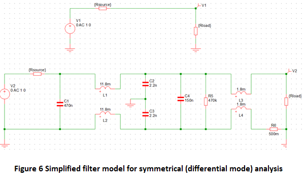
The filter insertion loss analysis can be easily performed using the SPICE based AC analysis tool. The simulation model is shown in Figure 6. Selected frequency sweep can be completed within seconds, and the insertion loss is plotted either using the simulation probe tool or simply using the equation of 20log(mag(V1/V2)).

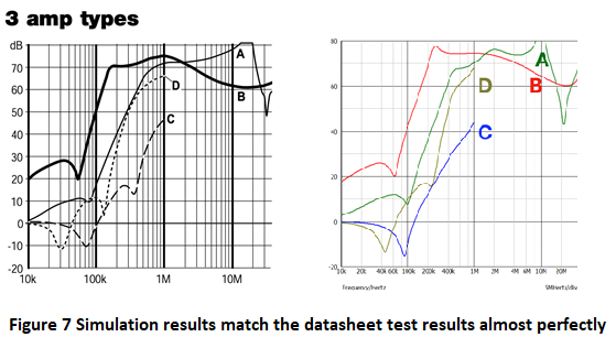
Figure 7 shows the simulated results compared with the datasheet measurement results. As it can be seen, a high level of matching is achieved.

Conclusion

In this article, the basics of filter insertion loss and measurement set-ups are introduced. Simulation model is presented to demonstrate the filter performance. The simulated insertion loss of the filter matches the test results very well.

« Back to Blog